Home → Air Quality → Programs → Meteorology Home → Permit Air Quality Modeling Guidelines → Class I Areas
Class I Analysis Preparation
Before preparing and submitting a Class I modeling protocol to MEDEP-BAQ (or beginning any modeling), it would very helpful to read and become familiar with recommendations and methodologies in the following documents:
• 2010 Federal Land Manager's AQRV Workgroup (FLAG) Report
• Interagency Workgroup on Air Quality Modeling (IWAQM) Phase 2 Summary Report for Modeling Long-Range Transport
• Guidance For Estimating Natural Visibility Conditions Under the regional Haze Rule (EPA-454/B-03-005)
Additional/updated Class I guiadnace can be found at the Federal Land Manager's AQRV webpage.
In addition, the CALPUFF modeling suite (CALPUFF, CALMET, CALPOST) and the associated utilities are available for download at no cost from the TRC website.
Class I Locations And AQRVs
For any major new source or any major modification (to an existing major or minor source), it is possible that a Class I increment and/or Air Quality Related Values (AQRVs) analyses will need to be performed, as required by the affected Federal Land Manager (FLM) of the 4 designated Class I areas in/near Maine. MEDEP-BAQ (the permitting authority) will work in close consultation with the FLMs and will ultimately be responsible for making the final determination regarding the Class I analyses.
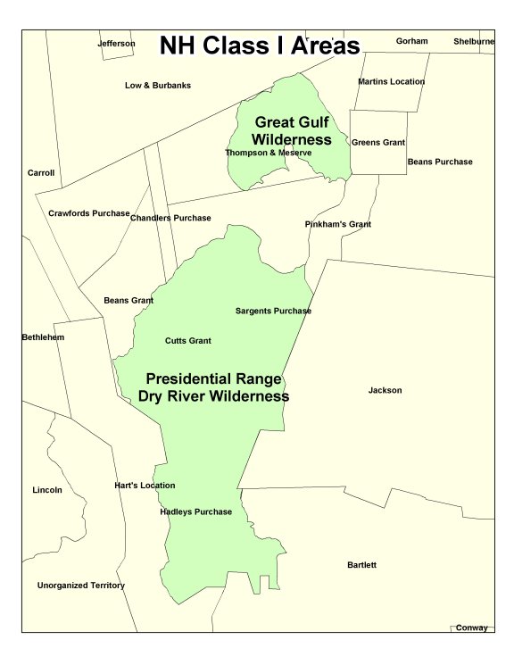
The locations of the four Class I areas can be found in the following maps:
 Acadia National Park |
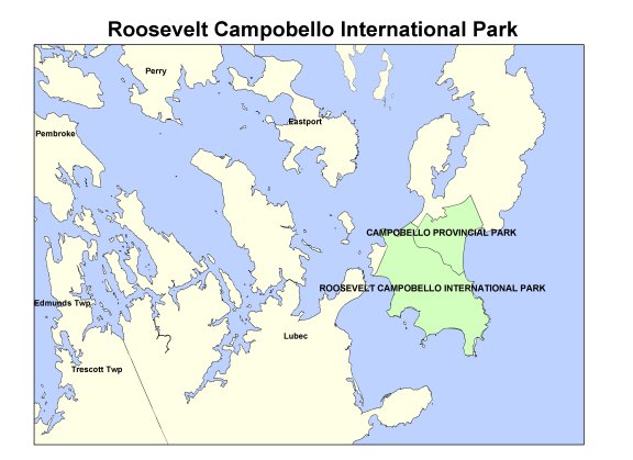 Roosevelt Campobello International Park |
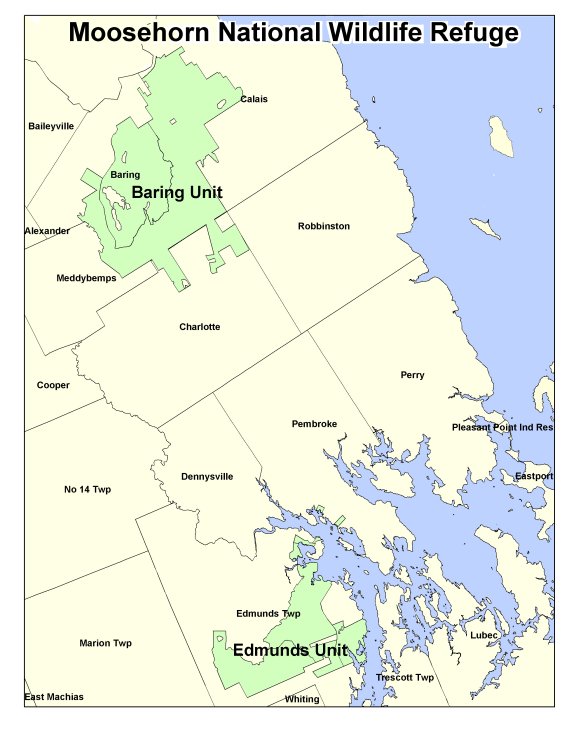 Moosehorn National Wildlife Refugee |
|
The FLM of each Class I area will make a determination as to the level of analysis necessary, if any, to evaluate increment and/or AQRVs. Potential AQRVs include: dry/wet deposition, visibility impacts, etc.
General information on AQRVs can be found at: http://www.nature.nps.gov/air/Permits/ARIS/aqrv.cfm
Proximity of Sources to Class I Areas
Should an FLM request any Class I increment and/or AQRV analyses, the model(s) and methodology will depend on the distance from the source to the affected Class I area. The modeled source will fall into one of the two following categories:
Sources within 50 kilometers of a Class I area
Sources beyond 50 kilometers of a Class I area
Sources Within 50 Kilometers of a Class I Area
To evaluate maximum concentrations, increments and/or dry/wet deposition impacts in Class I areas within 50 kilometers of the source, any EPA-approved near-field model (AERMOD-PRIME, etc.) may be used.
Near-field models and methodologies will be similar to those outlined in the "refined modeling" section of this document.
EPA and FLMs have recommended the use of the VISCREEN plume visibility model (EPA 1992b) for assessing potential plume visibility impacts in Class I areas within 50 kilometers of the source. PLUVUE II is also a recommended as a visibility model, but given that it is somewhat more difficult to run, it is typically applied only after using VISCREEN as a "first-cut" approach. Further guidance can be found in Workbook for Plume Visual Impact Screening and Analysis (Revised) (EPA, 1992).
Class I Receptors
Please contact the Department for assistance with obtaining information on Class I Receptors.
Additional information on these receptor grids is available from the National Park Service web site as well as the IWAQM Phase 2 and FLAG documents.
General Visibility Requirements
The potential for plume visibility impacts within these Class I areas must be assessed. Additionally, integral vistas have been defined for Acadia National Park and for Roosevelt Campobello International Park and the potential for plume visual impact on these integral vistas must also be assessed. Two criteria are used to screen for potential impact:
Delta-E (L*A*B) values greater than two (2.0); and
Plume contrast values of magnitude greater than 0.05
Delta-E (L*A*B) is a plume perceptibility parameter based on color differences and brightness. The plume contrast is a spectral criterion defined for a green wavelength of 0.55 microns.
The Workbook for Plume Visual Impact Screening and Analysis recommends the use of a plume visual impact screening model (VISCREEN) for two successive levels of screening (Levels 1 and 2) and may, on occasion, be applied to Level-3 screening as well. A detailed plume visual impact analysis (Level 3) can also be conducted using the more sophisticated plume visibility model, PLUVUE II.
VISCREEN
The VISCREEN model is an easy to use plume visibility screening model. The model is appropriate for Level-1 and Level-2 analyses, and may, on occasion, be applied to Level-3 screening as well.
Level-1 Analysis
Level-1 screening is the simplest and most direct. The user inputs total emissions from the source being modeled, specifies distances to the Class I area being assessed and appropriate background visual range value(s). Background visual range value(s) can be obtained from the FLM of each Class I area(s). Level-1 screening uses conservative default values for all other model parameters.
In order to completely assess potential plume impact on integral vistas and in those cases where such a geometry would carry the plume into a Class I area, a Level-1 analysis should also be made for plume-source-observer angles of 90º, 45º, and 22.5º. To do this, the user runs VISCREEN as in a Level-2 analysis, selects the change meteorology option and inputs the alternate plume-source-observer angle while using the Level-1 default values and screening criteria for all other parameters.
If a source fails to meet the Level-1 screening, a Level-2 analysis is required. When a Level-2 screening is performed, the user will input specific meteorological conditions, and may alter the geometry relating the plume, source, and observer, and other parameters.
Level-2 Analysis
Two methodologies are suggested for a Level-2 analysis. The first is specified in the VISCREEN workbook (EPA 1992b). The second is to use the VISCREEN model to define the envelope of wind speed and stability conditions within which VISCREEN predicts a delta-E(L*A*B) and/or plume contrast in excess of the screening criteria suggested. Section 4 of the VISCREEN workbook (EPA 1992b) contains guidance for determinations of the worst-case meteorological conditions.
Once these limiting meteorological conditions are defined, if a site-specific meteorological database is available, search that database for those conditions that might support a visible plume and which have reported winds that would transport the plume from the source to the Class I area.
Using the maximum wind speed found to support a visible plume, determine the minimum travel time to transport the plume from the source to the Class I area. Select from the hours that might support a visible plume only those events whose duration is sufficient for the plume to reach the Class I area. Further reduce the possible number of plume impact events by eliminating hours of darkness (defined as being between the end of evening civil twilight and the beginning of morning civil twilight) and any hours combining wind speeds and stabilities for which VISCREEN did not predict a potentially visible plume.
For sources located close to a Class I area and/or sources with especially large emission rates, the VISCREEN Level-2 analysis may still indicate the potential for plume visibility impacts. In this case a Level-3 analysis using perhaps both the VISCREEN and the PLUVUE II models may be necessary.
Level-3 Analysis
A Level-3 analysis forgoes the usual conservation of screening modelingand attempts to take a much more realistic look at the conditions that could lead to visual impacts in a Class I area. Such an analysis should seek to quantify the frequency of plume visual impact in the Class I area.
If a Level 3 analysis is required, any refined model should be selected in consultation with MEDEP, USEPA and the appropriate Federal Land Manager(s) to determine whether there is an adverse effect by a plume on a Class I area (EPA 1993a) and (EPA 1995a). Further guidance can be found in the VISCREEN workbook (EPA 1992b)
Additional guidance on the VISCREEN can be found in the Dispersion Models section of the SCRAM website.
PLUVUE II
A detailed plume visual impact analysis (Level 3) can be conducted using the more sophisticated plume visibility model, PLUVUE II.
PLUVUE II is a detailed model used for estimating visual range reduction and atmospheric discoloration caused by plumes resulting from the emissions of particles, nitrogen oxides and sulfur oxides from a single emission source. PLUVUE II predicts the transport, dispersion, chemical reactions, optical effects and surface deposition of point or area source emissions.
It is recommended to read: User's Manual for the Plume Visibility Model (PLUVUE II) (EPA, 1984a and EPA, 1984b) before any modeling begins.
Additional guidance on PLUVUE II can be found in the Dispersion Models section of the SCRAM website.
Sources Beyond 50 Kilometers of a Class I Area
Close consultation with MEDEP-BAQ and the appropriate Federal Land Managers (FLMs) is highly recommended to determine the best methods for estimating long range (> 50km) impacts of regulated pollutants on Class I areas, impacts on air quality related values (AQRVs) and impacts on regional visibility. Until more concrete guidance is issued on these subjects, the most recent recommendations from the following documents shall be considered on a case-by-case basis:
• 2010 Federal Land Manager's AQRV Workgroup (FLAG) Report
• Interagency Workgroup on Air Quality Modeling (IWAQM) Phase 2 Summary Report for Modeling Long-Range Transport
It is important to note that CALPUFF is the only EPA-approved (Appendix W) model to be used for source-receptor distances of greater than 50 kilometers. Due to the tremendous complexity of running the CALPUFF model in refined mode, it would be very difficult to provide project-specific modeling guidance. At this time, only basic CALPUFF guidance is included in this document.
NOTE: Only modelers who have obtained proper training should attempt to model using CALPUFF. Proper CALPUFF training will be the key in submitting an accurate and cost effective modeling analysis for the applicant. As stated prviously, MEDEP-BAQ is available as a resource for project-specific questions, however, MEDEP-BAQ will not provide training in the use of air quality models.
CALPUFF Modeling Protocol/Submittals
Due to complexity of the CALPUFF model, all sections of the CALPUFF protocol/modeling report should contain sufficient detail as to allow other modelers to replicate the analysis while fully understanding the rational behind model selection and application. Simply providing all input/output/diagnostic files on CD/flashdrive will not be considered acceptable. All submittals should demonstrate to the project meteorologist, USEPA and the affected FLM(s) that the model inputs were developed correctly and that the model has been applied properly.
Meteorological Data
The modeling protocol should include a detailed description and justification of the meteorological data selected/processed, as well as the justification for all parameters.
It is very important that you work in conjunction with the project meteorologist when developing your meteorological data files, to resolve any issues during (and not after) the processing of the database.
Class I ReceptorsPlease contact the Department for assistance with obtaining information on Class I Receptors.
Additional information on these receptor grids is available from the National Park Service web site as well as the IWAQM Phase 2 and FLAG documents.
General CALPUFF Notes
CALPUFF does NOT accept negative emission rates (for increment runs). There is a utility (POSTUTIL.EXE) that will correctly post-process the CALPUFF-LITE runs to account for emissions sources existing in the baseline year(s). This utility is available on TRC's website.
General CALPOST Notes
Extinction values for hygroscopic and non-hygroscopic aerosols are to be derived from the tables listed in the FLAG report. CALPOST does not explicitly allow for the direct input of hygroscopic and non-hygroscopic to extinction, it only allows for the concentration of a particular species. Since the FLAG report has the individual components already combined, it is necessary to "back out" the concentration from the extinction provided:
• To account for non-hygroscopic pollutants, enter the non-hygroscopic extinction values (either seasonal or annual) that are listed in the FLAG report tables into CALPOST as "Monthly Background Concentrations" into the SOIL (BKSOIL) variable.
• For hygroscopic pollutants, divide the values given in the FLAG report by 3 (the extinction efficiency of sulfates and nitrates), and then enter that hygroscopic extinction value into the AMMONIUM SULFATE (BKSO4) variable for all 12 months.
AQRV analyses typically require that the total sulfur and nitrogen deposition be calculated in a particular Class I area. Since the dry and wet deposition estimates contain oxides of both sulfur and nitrogen, the CALPOST results must be adjusted for the difference in molecular weight of their oxides and the element. The normalized results can then be summed to yield the total sulfur and/or nitrogen deposition.
This can be done in one of two ways:
Method 1
When using CALPOST for dry and/or wet deposition calculations, the following pollutants will need to be considered in the total deposition:
• For dry deposition calculations, process: SO2, SO4, NOx, HNO3, NO3
• For wet deposition calculations, process: SO2, SO4, HNO3, NO3Be sure to make a separate CALPOST deposition run for each pollutant (dry and wet, for a total of 9 CALPOST files per year of meteorological data) from the individual *.DRY and *.WET CALPUFF output files. Next, adjust each specie (listed above) to account for the different molecular weight (See IWAQM, Page 31). Finally, the normalized individual sulfur and nitrogen estimates can then be summed to generate the final predicted deposition value. This is likely to be best handled through the use of a spreadsheet.
Method 2The POSTUTIL.EXE program can be used to automatically perform the steps outlined in Method 1. Use the *.DRY and *.WET output files created by CALPUFF as input files for the POSTUTIL.EXE utility. POSTUTIL.EXE will generate 2 files, *.LST (diagnostic file) and *.DEP (deposition file). When running the program, specify the species that you need depositions estimates for, in this case, sulfur and nitrogen. Finally, run CALPOST two times using the *.DEP file, once for the total sulfur deposition and once for the total nitrogen deposition.